The volatile and complex nature of cryptocurrency markets presents both challenges and opportunities for algorithmic trading. Reinforcement learning (RL) offers a powerful framework for developing adaptive trading strategies that can navigate this complexity. Unlike traditional technical analysis or supervised learning approaches, RL agents learn by interacting with the market environment, optimizing their strategies through trial and error. This guide will walk you through the process of implementing reinforcement learning for cryptocurrency trading strategy optimization, from fundamental concepts to practical implementation.
Fundamentals of Reinforcement Learning for Crypto Trading
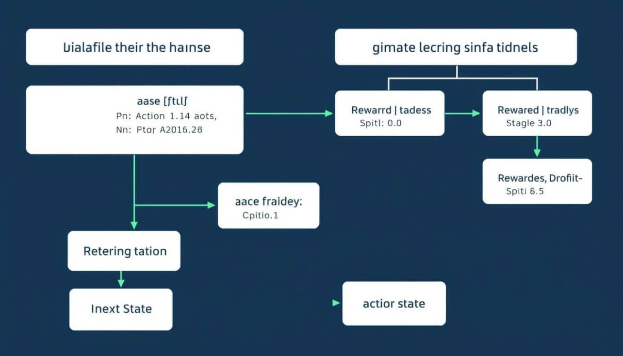
Reinforcement Learning Framework for Cryptocurrency Trading
Reinforcement learning is a branch of machine learning where an agent learns to make decisions by taking actions in an environment to maximize cumulative rewards. In the context of cryptocurrency trading, the agent is your trading algorithm, the environment is the market, actions are trading decisions (buy, sell, hold), and rewards are typically based on profit or risk-adjusted returns.
Key Components of RL in Crypto Trading
Agent
The trading algorithm that learns to make decisions. It observes the market state (prices, volumes, technical indicators) and executes actions based on its policy. The agent’s goal is to maximize cumulative rewards over time by optimizing its trading strategy.
Environment
The cryptocurrency market where the agent operates. The environment provides observations (market data) to the agent and returns rewards based on the agent’s actions. The crypto market environment is particularly challenging due to its high volatility, 24/7 operation, and non-stationary nature.
State
The market conditions observed by the agent at each time step. This typically includes price data, technical indicators, order book information, and the agent’s current portfolio state. The state representation is crucial for the agent’s ability to learn effective strategies.
Action
Trading decisions made by the agent, such as buying, selling, or holding assets. Actions can be discrete (e.g., buy/sell/hold) or continuous (e.g., percentage of portfolio to allocate). The action space design significantly impacts the complexity of the learning problem.
Reward
The feedback signal that guides the agent’s learning process. In crypto trading, rewards are typically based on profit/loss, but can also incorporate risk metrics like the Sharpe ratio or drawdown penalties. Designing an appropriate reward function is one of the most critical aspects of RL for trading.
Why Reinforcement Learning for Crypto Trading?
Advantages
- Adapts to changing market conditions without explicit reprogramming
- Optimizes directly for financial objectives rather than prediction accuracy
- Can learn complex non-linear strategies that traditional methods might miss
- Handles sequential decision-making under uncertainty
- Balances exploration of new strategies with exploitation of known profitable patterns
Challenges
- Requires careful environment design to avoid overfitting to historical data
- Training can be computationally intensive and time-consuming
- Reward function design is complex and impacts strategy development
- Market non-stationarity can lead to strategy degradation over time
- Difficult to interpret the learned strategies (black-box nature)
Setting Up a Cryptocurrency Trading Environment
Before implementing reinforcement learning algorithms, you need to create a suitable environment that simulates cryptocurrency trading. This environment will serve as the training ground for your RL agent.
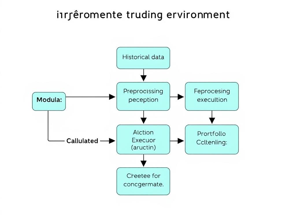
Components of a Cryptocurrency Trading Environment for RL
Creating a Custom Trading Environment
The first step is to create a custom environment that follows the OpenAI Gym interface, which is the standard for RL implementations. This environment should handle market data, execute trading actions, calculate rewards, and track the agent’s portfolio.
“`python
# Example: Custom RL environment for crypto trading
import gym
import numpy as np
from gym import spaces
class CryptoTradingEnv(gym.Env):
def __init__(self, df, initial_balance=10000, transaction_fee=0.001):
super(CryptoTradingEnv, self).__init__()
# Market data
self.df = df
self.current_step = 0
# Account information
self.initial_balance = initial_balance
self.balance = initial_balance
self.crypto_held = 0
self.transaction_fee = transaction_fee
# Define action and observation space
# Actions: 0 (HOLD), 1 (BUY), 2 (SELL)
self.action_space = spaces.Discrete(3)
# Observation space: OHLCV data + technical indicators + account state
self.observation_space = spaces.Box(
low=-np.inf, high=np.inf, shape=(self.df.shape[1] + 2,), dtype=np.float32
)
def reset(self):
self.current_step = 0
self.balance = self.initial_balance
self.crypto_held = 0
return self._get_observation()
def step(self, action):
# Execute action
self._take_action(action)
# Move to next time step
self.current_step += 1
# Calculate reward
reward = self._calculate_reward()
# Check if episode is done
done = self.current_step >= len(self.df) – 1
# Get next observation
obs = self._get_observation()
return obs, reward, done, {}
def _get_observation(self):
# Current market data
market_data = self.df.iloc[self.current_step].values
# Account state
account_state = np.array([
self.balance / self.initial_balance, # Normalized balance
self.crypto_held * self.df.iloc[self.current_step][‘close’] / self.initial_balance # Normalized position value
])
# Combine market data and account state
return np.concatenate([market_data, account_state])
def _take_action(self, action):
current_price = self.df.iloc[self.current_step][‘close’]
if action == 1: # BUY
# Calculate maximum crypto that can be bought
max_crypto = self.balance / (current_price * (1 + self.transaction_fee))
# Buy 100% of possible crypto
crypto_bought = max_crypto
cost = crypto_bought * current_price * (1 + self.transaction_fee)
self.balance -= cost
self.crypto_held += crypto_bought
elif action == 2: # SELL
# Sell all crypto
crypto_sold = self.crypto_held
revenue = crypto_sold * current_price * (1 – self.transaction_fee)
self.balance += revenue
self.crypto_held = 0
def _calculate_reward(self):
# Calculate portfolio value
current_price = self.df.iloc[self.current_step][‘close’]
portfolio_value = self.balance + self.crypto_held * current_price
# Calculate reward as change in portfolio value
prev_portfolio_value = self.balance + self.crypto_held * self.df.iloc[max(0, self.current_step-1)][‘close’]
reward = (portfolio_value – prev_portfolio_value) / self.initial_balance
return reward
“`
Data Preparation for RL Trading
High-quality data is essential for training effective RL trading agents. You’ll need to collect and preprocess historical cryptocurrency data, including price, volume, and potentially order book information.
Data Collection
Gather historical cryptocurrency data from reliable sources such as exchange APIs (Binance, Coinbase), data providers (CryptoCompare, Kaiko), or public datasets. Ensure your data includes at least OHLCV (Open, High, Low, Close, Volume) information at your desired time interval (e.g., 1-minute, 15-minute, 1-hour).
Feature Engineering
Create relevant technical indicators that can help your agent identify trading opportunities. Common indicators include Moving Averages (MA), Relative Strength Index (RSI), Bollinger Bands, MACD, and volume-based indicators. Normalize all features to ensure stable training.
Data Preprocessing
Clean the data by handling missing values, removing outliers, and ensuring consistency. Normalize or standardize features to have similar scales, which helps the learning algorithm converge faster. Split your data into training, validation, and testing sets, ensuring no look-ahead bias.
Market Simulation
Implement realistic market dynamics in your environment, including transaction fees, slippage, and liquidity constraints. These factors significantly impact real-world trading performance and should be accounted for during training.
“`python
# Example: Data preprocessing for RL trading
import pandas as pd
import numpy as np
import ta
def preprocess_data(df):
# Calculate technical indicators
# Trend indicators
df[‘sma_7’] = ta.trend.sma_indicator(df[‘close’], window=7)
df[‘sma_25’] = ta.trend.sma_indicator(df[‘close’], window=25)
df[‘macd’] = ta.trend.macd_diff(df[‘close’])
# Momentum indicators
df[‘rsi’] = ta.momentum.rsi(df[‘close’])
# Volatility indicators
bollinger = ta.volatility.BollingerBands(df[‘close’])
df[‘bollinger_pct’] = bollinger.bollinger_pband()
# Volume indicators
df[‘volume_adi’] = ta.volume.acc_dist_index(df[‘high’], df[‘low’], df[‘close’], df[‘volume’])
# Fill NaN values
df.fillna(method=’bfill’, inplace=True)
# Normalize features
for column in df.columns:
if column != ‘timestamp’:
df[column] = (df[column] – df[column].mean()) / df[column].std()
return df
“`
Ready to Start Building Your RL Trading Environment?
Get access to our complete GitHub repository with ready-to-use code for setting up custom cryptocurrency trading environments, data preprocessing pipelines, and example RL implementations.
Designing Effective Reward Functions
The reward function is perhaps the most critical component of your reinforcement learning system for cryptocurrency trading. It defines what your agent optimizes for and directly shapes the learned trading strategy.
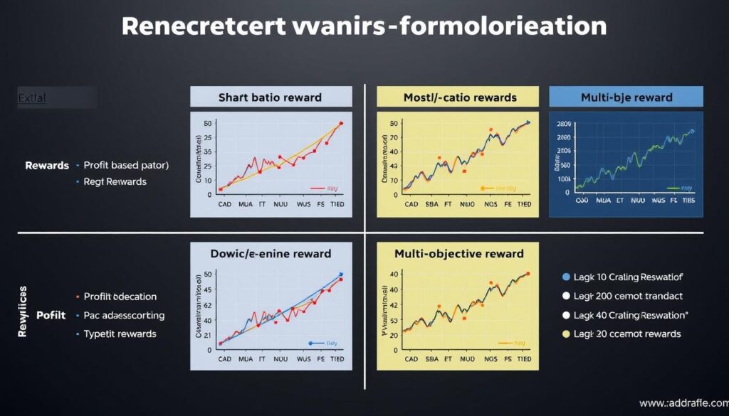
Comparison of Different Reward Functions for RL Trading Strategies
Common Reward Functions for Crypto Trading
| Reward Type | Formula | Advantages | Disadvantages |
| Profit-Based | R = (portfolio_value_t – portfolio_value_t-1) / initial_capital | Direct optimization for profit, intuitive, easy to implement | May lead to excessive risk-taking, doesn’t account for volatility |
| Sharpe Ratio | R = (mean_return – risk_free_rate) / std_deviation | Balances return and risk, industry-standard metric | Assumes normal distribution of returns, penalizes upside volatility |
| Sortino Ratio | R = (mean_return – risk_free_rate) / downside_deviation | Only penalizes downside risk, better for asymmetric returns | More complex to implement, requires downside deviation calculation |
| Drawdown-Penalized | R = profit – λ * max_drawdown | Explicitly manages drawdown risk, more conservative strategies | Requires tuning of penalty coefficient λ |
| Multi-Objective | R = w₁*profit + w₂*sharpe + w₃*turnover_penalty | Flexible, can optimize for multiple objectives simultaneously | Requires careful weight tuning, potential objective conflicts |
Implementing Reward Functions
“`python
# Example: Different reward function implementations
# 1. Simple profit-based reward
def profit_reward(env):
current_price = env.df.iloc[env.current_step][‘close’]
portfolio_value = env.balance + env.crypto_held * current_price
prev_portfolio_value = env.balance + env.crypto_held * env.df.iloc[max(0, env.current_step-1)][‘close’]
return (portfolio_value – prev_portfolio_value) / env.initial_balance
# 2. Sharpe ratio reward (using rolling window)
def sharpe_reward(env, window=30, risk_free_rate=0):
if env.current_step Reward Function Design Tips
Balancing Short and Long-term Rewards: Use a discount factor (gamma) to balance immediate returns with long-term profitability. A higher gamma (closer to 1) makes the agent more forward-looking.
Avoid Reward Hacking: Ensure your reward function can’t be exploited by unintended agent behaviors. For example, if you only reward profits without penalizing risk, the agent might learn to take excessive risks.
When designing your reward function, consider your trading objectives and risk tolerance. A profit-maximizing reward might be suitable for aggressive strategies, while a Sharpe ratio or drawdown-penalized reward would be better for risk-conscious approaches. You can also combine multiple reward components with appropriate weights to create a custom reward function that aligns with your specific trading goals.
Selecting Appropriate RL Algorithms
Different reinforcement learning algorithms have varying strengths and weaknesses when applied to cryptocurrency trading. The choice of algorithm depends on your specific requirements, computational resources, and the complexity of your trading strategy.
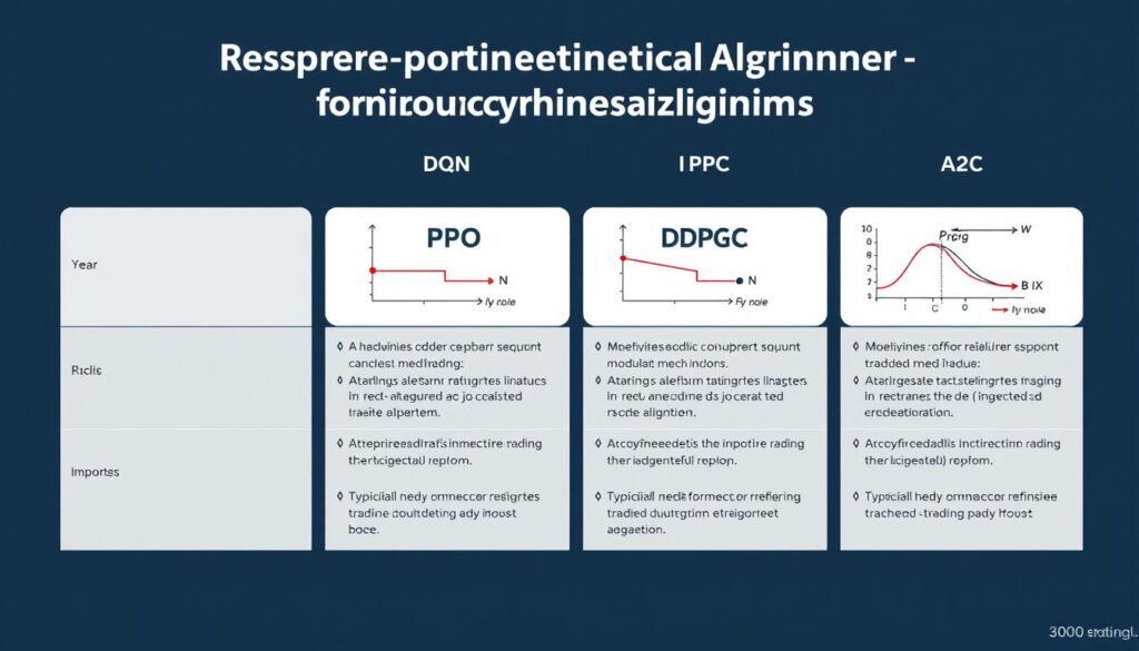
Comparison of RL Algorithms for Cryptocurrency Trading
Popular RL Algorithms for Crypto Trading
Deep Q-Network (DQN)
Value-Based Discrete Actions
DQN combines Q-learning with deep neural networks to approximate the action-value function. It’s suitable for discrete action spaces (buy/sell/hold) and uses experience replay and target networks to stabilize training.
Best for: Simple trading strategies with discrete actions and smaller state spaces.
Proximal Policy Optimization (PPO)
Policy-Based Discrete/Continuous
PPO is a policy gradient method that optimizes policies directly while ensuring the new policy doesn’t deviate too much from the old one. It’s known for its stability and sample efficiency.
Best for: Complex trading strategies requiring robust performance across different market conditions.
Deep Deterministic Policy Gradient (DDPG)
Actor-Critic Continuous Actions
DDPG combines policy gradient and Q-learning approaches, making it suitable for continuous action spaces. It can learn policies for determining exact position sizes or allocation percentages.
Best for: Portfolio allocation and position sizing strategies requiring precise control.
Advantage Actor-Critic (A2C/A3C)
Actor-Critic Discrete/Continuous
A2C maintains both value and policy networks, using the advantage function to reduce variance in policy updates. A3C extends this with parallel training across multiple environments.
Best for: Efficient training with limited computational resources.
Soft Actor-Critic (SAC)
Actor-Critic Continuous Actions
SAC is an off-policy actor-critic algorithm that incorporates entropy maximization to encourage exploration. It’s particularly effective in environments with multiple viable strategies.
Best for: Exploring diverse trading strategies in uncertain market conditions.
Twin Delayed DDPG (TD3)
Actor-Critic Continuous Actions
TD3 addresses overestimation bias in DDPG by using twin Q-networks and delayed policy updates. It provides more stable learning for continuous control problems.
Best for: Precise position sizing with improved stability over DDPG.
Implementing PPO for Crypto Trading
Proximal Policy Optimization (PPO) is often a good starting point for cryptocurrency trading due to its stability and sample efficiency. Here’s an example implementation using the Stable Baselines3 library:
“`python
# Example: Implementing PPO for crypto trading
import gym
import numpy as np
from stable_baselines3 import PPO
from stable_baselines3.common.vec_env import DummyVecEnv
# Assuming CryptoTradingEnv is already defined
# Prepare the environment
df = preprocess_data(load_crypto_data())
env = CryptoTradingEnv(df)
env = DummyVecEnv([lambda: env])
# Define the model
model = PPO(
policy=”MlpPolicy”,
env=env,
learning_rate=0.0003,
n_steps=2048,
batch_size=64,
n_epochs=10,
gamma=0.99,
gae_lambda=0.95,
clip_range=0.2,
clip_range_vf=None,
ent_coef=0.01,
vf_coef=0.5,
max_grad_norm=0.5,
verbose=1
)
# Train the model
model.learn(total_timesteps=1000000)
# Save the model
model.save(“ppo_crypto_trader”)
# Test the model
obs = env.reset()
for i in range(len(df) – 1):
action, _states = model.predict(obs)
obs, rewards, dones, info = env.step(action)
if dones:
break
“`
Algorithm Selection Guidelines
Consider Your Action Space
For discrete actions (buy/sell/hold), algorithms like DQN, PPO, or A2C work well. For continuous actions (position sizing, portfolio allocation percentages), consider DDPG, TD3, or SAC.
Sample Efficiency
If you have limited computational resources or training data, prioritize sample-efficient algorithms like PPO or SAC. Off-policy algorithms (DQN, DDPG, SAC) can reuse past experiences, making them more data-efficient than on-policy methods (A2C, vanilla policy gradient).
Stability vs. Performance
Some algorithms offer better stability (PPO, TD3) while others might achieve higher performance but with more tuning required (SAC, DDPG). For production systems, stability is often more important than squeezing out marginal performance gains.
Exploration Requirements
Markets with clear patterns may require less exploration, while highly volatile or unpredictable markets benefit from algorithms with strong exploration mechanisms (SAC with entropy maximization or noisy networks).
Accelerate Your RL Trading Development
Download our pre-configured RL trading framework with implementations of all major algorithms optimized for cryptocurrency markets.
Optimization Techniques for RL Trading Strategies
Developing effective reinforcement learning trading strategies requires careful optimization beyond just algorithm selection. This section covers essential techniques to improve your RL trading system’s performance and robustness.
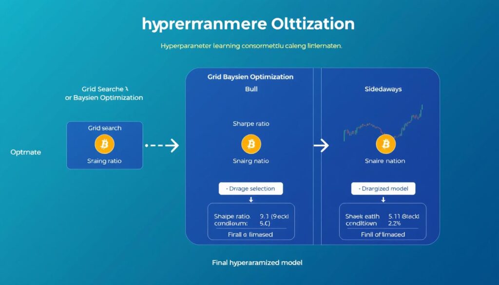
Hyperparameter Optimization Process for RL Trading Strategies
Hyperparameter Tuning
Hyperparameter optimization is crucial for RL trading strategies, as performance can vary significantly based on parameter choices. Here are key hyperparameters to tune:
Learning Parameters
- Learning rate: Controls how quickly the model adapts to new information
- Batch size: Number of samples used for each training update
- Discount factor (gamma): Balances immediate vs. future rewards
- Exploration parameters: Epsilon decay rate, entropy coefficient
Network Architecture
- Network depth: Number of hidden layers
- Layer width: Neurons per hidden layer
- Activation functions: ReLU, tanh, etc.
- Regularization: Dropout rate, L2 penalty
Environment Parameters
- Reward scaling: Magnitude of rewards
- State normalization: Feature scaling methods
- Action frequency: Trading interval (hourly, daily)
- Transaction costs: Fee structure modeling
“`python
# Example: Hyperparameter tuning with Optuna
import optuna
from stable_baselines3 import PPO
from stable_baselines3.common.evaluation import evaluate_policy
def objective(trial):
# Define hyperparameters to optimize
learning_rate = trial.suggest_float(“learning_rate”, 1e-5, 1e-3, log=True)
n_steps = trial.suggest_int(“n_steps”, 1024, 4096)
batch_size = trial.suggest_int(“batch_size”, 32, 256)
gamma = trial.suggest_float(“gamma”, 0.9, 0.9999)
ent_coef = trial.suggest_float(“ent_coef”, 0.00001, 0.1, log=True)
# Create environment
env = DummyVecEnv([lambda: CryptoTradingEnv(train_df)])
eval_env = DummyVecEnv([lambda: CryptoTradingEnv(val_df)])
# Create and train model
model = PPO(
policy=”MlpPolicy”,
env=env,
learning_rate=learning_rate,
n_steps=n_steps,
batch_size=batch_size,
gamma=gamma,
ent_coef=ent_coef,
verbose=0
)
model.learn(total_timesteps=100000)
# Evaluate model
mean_reward, _ = evaluate_policy(model, eval_env, n_eval_episodes=10)
return mean_reward
# Run optimization
study = optuna.create_study(direction=”maximize”)
study.optimize(objective, n_trials=50)
# Get best parameters
best_params = study.best_params
print(f”Best parameters: {best_params}”)
print(f”Best value: {study.best_value}”)
“`
Backtesting and Validation
Proper backtesting is essential to evaluate your RL trading strategy’s performance across different market conditions. Implement these practices for robust validation:
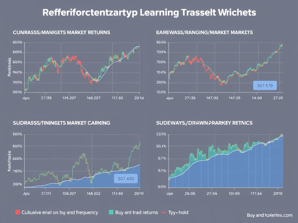
Backtesting RL Trading Strategies Across Different Market Conditions
Walk-Forward Validation
Use walk-forward validation to simulate real-world trading conditions. Train on a historical period, validate on the subsequent period, then move the window forward and repeat. This approach helps assess how well your strategy adapts to changing market conditions over time.
Market Regime Testing
Test your strategy across different market regimes: bull markets, bear markets, sideways/ranging markets, and high-volatility periods. A robust strategy should perform reasonably well across various conditions or at least avoid significant losses in unfavorable environments.
Out-of-Sample Testing
Always evaluate your strategy on data that was not used during training or hyperparameter tuning. This helps detect overfitting and provides a more realistic estimate of real-world performance. Consider testing on different cryptocurrencies than those used for training.
Benchmark Comparison
Compare your strategy against benchmarks like buy-and-hold, traditional technical indicators, or simpler algorithms. This provides context for evaluating performance and helps identify the value added by your RL approach.
Risk Management Integration
Effective risk management is crucial for long-term trading success. Integrate these risk management techniques into your RL trading system:
Position Sizing
Implement dynamic position sizing based on market volatility and confidence levels. This can be learned by the RL agent or implemented as a post-processing step. Kelly criterion or volatility-adjusted position sizing can help optimize risk-reward balance.
Stop-Loss Mechanisms
Incorporate automatic stop-loss mechanisms to limit potential losses. These can be fixed percentage stops, volatility-based stops (e.g., ATR-based), or learned by the agent as part of its policy. Stop-losses are especially important in the volatile crypto market.
Drawdown Control
Implement maximum drawdown constraints that temporarily halt trading when drawdown exceeds predefined thresholds. This prevents catastrophic losses during adverse market conditions and allows the strategy to preserve capital for better opportunities.
“`python
# Example: Implementing stop-loss and take-profit in the environment
def _take_action(self, action):
current_price = self.df.iloc[self.current_step][‘close’]
# Track entry price when opening a position
if action == 1 and self.crypto_held == 0: # BUY
max_crypto = self.balance / (current_price * (1 + self.transaction_fee))
crypto_bought = max_crypto
cost = crypto_bought * current_price * (1 + self.transaction_fee)
self.balance -= cost
self.crypto_held += crypto_bought
self.entry_price = current_price
elif action == 2 or self._check_stop_loss_take_profit(): # SELL or stop triggered
crypto_sold = self.crypto_held
revenue = crypto_sold * current_price * (1 – self.transaction_fee)
self.balance += revenue
self.crypto_held = 0
self.entry_price = 0
def _check_stop_loss_take_profit(self):
if self.crypto_held == 0:
return False
current_price = self.df.iloc[self.current_step][‘close’]
profit_pct = (current_price – self.entry_price) / self.entry_price
# Stop loss: 5% loss
if profit_pct = 0.15:
return True
return False
“`
Overfitting Warning: Reinforcement learning agents are particularly prone to overfitting to historical data patterns. Always validate on out-of-sample data and implement robust risk management to mitigate this risk.
Case Study: BTC/ETH Trading Bot
Let’s examine a real-world implementation of a reinforcement learning trading bot for the BTC/USD and ETH/USD markets. This case study demonstrates the practical application of the concepts covered in this guide.
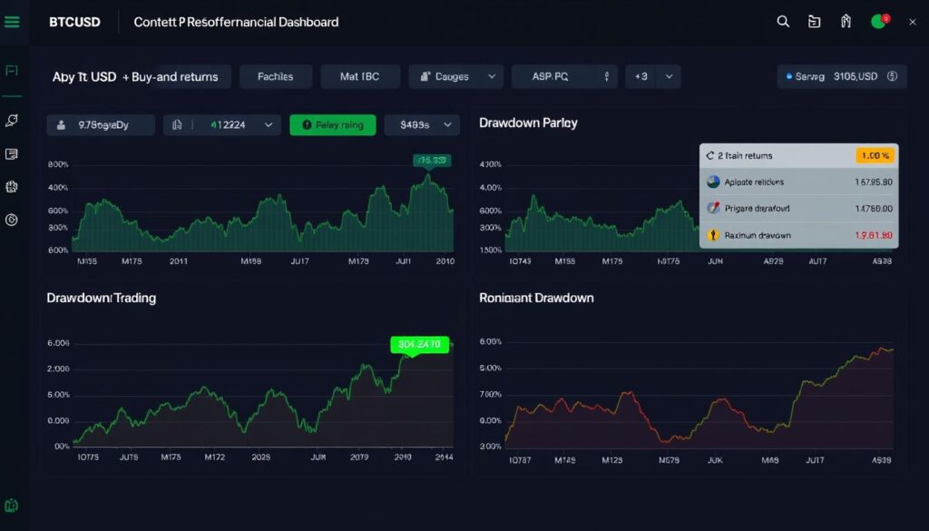
Performance Dashboard of RL Trading Bot for BTC/USD and ETH/USD
Implementation Details
Environment Setup
The trading environment was implemented using the OpenAI Gym interface with 1-hour OHLCV data from Binance for BTC/USD and ETH/USD pairs. The state space included 24 technical indicators, recent price action, and current position information. The action space was discrete with three actions: buy, sell, and hold.
Algorithm Selection
After testing multiple algorithms, PPO (Proximal Policy Optimization) was selected for its stability and sample efficiency. The neural network architecture consisted of three fully connected layers with 128, 64, and 32 neurons respectively, using ReLU activations and a final softmax layer for action probabilities.
Reward Function
A multi-objective reward function was implemented, combining profit-based rewards with a Sharpe ratio component and drawdown penalties:
reward = 0.6 * profit_pct + 0.3 * sharpe_contribution - 0.1 * drawdown_penalty
This balanced approach encouraged the agent to seek profitable trades while managing risk and avoiding excessive drawdowns.
Risk Management
The strategy incorporated a 2% per-trade risk limit and implemented dynamic position sizing based on the agent’s confidence (action probabilities). Additionally, a 15% maximum drawdown circuit breaker was implemented to pause trading during severe market downturns.
Performance Results
| Metric | BTC/USD | ETH/USD | Buy-and-Hold (BTC) |
| Annual Return | 32.4% | 41.7% | 27.8% |
| Sharpe Ratio | 1.85 | 1.92 | 0.98 |
| Maximum Drawdown | 18.3% | 22.1% | 53.4% |
| Win Rate | 62.7% | 58.9% | N/A |
| Profit Factor | 1.87 | 1.73 | N/A |
Key Insights and Lessons
Market Adaptation
The RL agent demonstrated an impressive ability to adapt to changing market conditions. During the backtesting period, which included both bull and bear markets, the agent learned to increase position sizes during uptrends and reduce exposure during downtrends.
Volatility Management
The multi-objective reward function successfully encouraged the agent to manage volatility. The strategy achieved significantly lower drawdowns compared to buy-and-hold while maintaining competitive returns, resulting in superior risk-adjusted performance.
Training Challenges
Initial training attempts suffered from overfitting to specific market regimes. This was addressed by implementing curriculum learning, starting with simple market conditions and gradually introducing more complex scenarios, which significantly improved generalization.
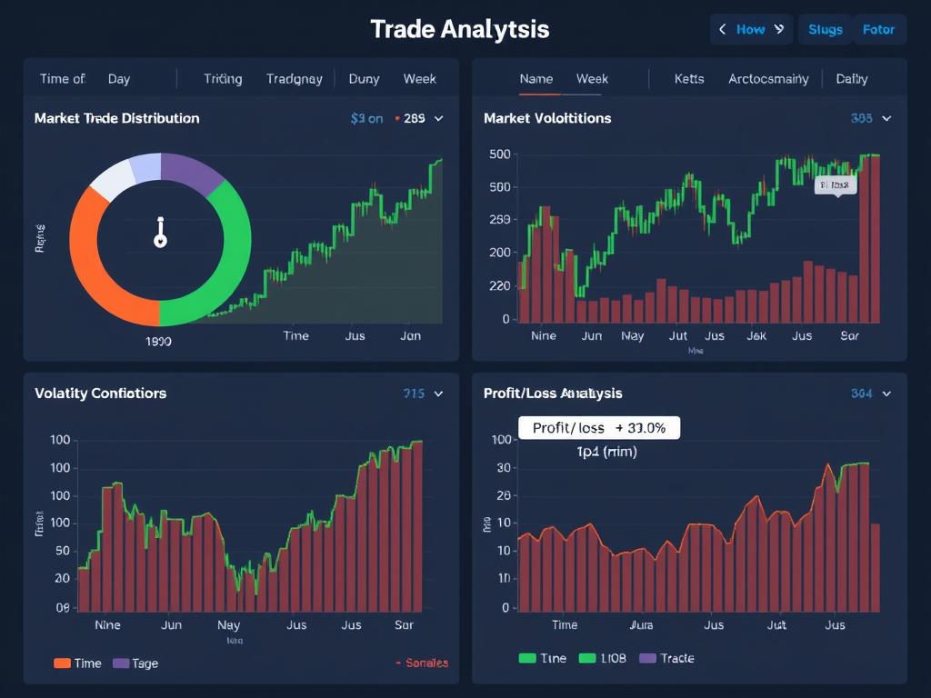
Trade Distribution Analysis of the RL Trading Strategy
This case study demonstrates that reinforcement learning can develop effective cryptocurrency trading strategies that outperform simple benchmarks on a risk-adjusted basis. The key to success was the combination of appropriate algorithm selection, careful environment design, multi-objective reward engineering, and robust risk management integration.
Frequently Asked Questions
Can reinforcement learning handle sudden cryptocurrency market crashes?
Reinforcement learning agents can be trained to handle market crashes, but their effectiveness depends on several factors:
- Training data exposure: If the agent has been trained on historical data that includes crashes, it may learn appropriate responses.
- Reward function design: Incorporating drawdown penalties and risk-adjusted metrics in the reward function encourages the agent to develop risk management strategies.
- Explicit risk controls: Implementing stop-loss mechanisms and maximum drawdown limits as part of the environment provides additional protection.
For best results, combine RL with traditional risk management techniques like position sizing, stop-losses, and circuit breakers to provide safeguards during extreme market events.
Which cryptocurrencies work best with RL trading strategies?
RL trading strategies tend to perform better on cryptocurrencies with the following characteristics:
- High liquidity: Major cryptocurrencies like BTC and ETH have sufficient liquidity to execute trades with minimal slippage.
- Sufficient volatility: Some price movement is necessary for the agent to find profitable trading opportunities.
- Longer history: More historical data allows for better training and validation.
- Lower correlation: Cryptocurrencies with unique price patterns provide diversification benefits.
Bitcoin and Ethereum are good starting points due to their liquidity and data availability. Mid-cap altcoins can also work well but may require more careful risk management due to higher volatility and lower liquidity.
How much historical data is needed to train an effective RL trading agent?
The amount of historical data needed depends on several factors:
- Trading frequency: Higher frequency strategies (hourly, minute-level) require more data points than lower frequency strategies (daily, weekly).
- Market cycles: Ideally, your training data should include different market regimes (bull, bear, sideways).
- Algorithm complexity: More complex models with many parameters require more data to avoid overfitting.
As a general guideline, aim for at least 2-3 years of historical data for daily strategies and 6+ months for hourly strategies. For minute-level data, several weeks to months may be sufficient. Quality matters more than quantity—ensure your data covers diverse market conditions.
How do you handle the non-stationarity of cryptocurrency markets in RL?
Cryptocurrency markets are non-stationary, meaning their statistical properties change over time. To address this challenge:
- Continuous learning: Implement online learning where the agent continues to adapt in production.
- Adaptive feature engineering: Use relative or normalized features rather than absolute values.
- Ensemble approaches: Train multiple agents on different market regimes and combine their predictions.
- Meta-learning: Train the agent to quickly adapt to new market conditions with minimal data.
- Regime detection: Incorporate market regime detection to switch between specialized policies.
Regular retraining on recent data is also essential to keep the agent updated with evolving market dynamics.
What computational resources are required for RL trading strategy development?
Resource requirements vary based on your implementation:
- Basic setup: A modern laptop with 16GB RAM and a decent CPU can handle simple RL implementations with daily or hourly data.
- Mid-range setup: For faster training and more complex models, a desktop with a good GPU (e.g., NVIDIA RTX series), 32GB RAM, and a multi-core CPU is recommended.
- Advanced setup: For high-frequency strategies or extensive hyperparameter tuning, consider cloud-based solutions with multiple GPUs or TPUs.
Cloud platforms like Google Colab Pro, AWS SageMaker, or Azure ML provide cost-effective options for training resource-intensive models without investing in expensive hardware.
Ready to Implement Your Own RL Trading Strategy?
Get access to our complete reinforcement learning trading framework, including pre-built environments, optimized algorithms, and example strategies for major cryptocurrencies.
Conclusion
Reinforcement learning offers a powerful framework for developing adaptive cryptocurrency trading strategies that can navigate the complexity and volatility of digital asset markets. By directly optimizing for financial objectives rather than prediction accuracy, RL approaches can potentially outperform traditional trading methods, especially in rapidly changing market conditions.
This guide has covered the essential components of implementing RL for cryptocurrency trading: setting up appropriate trading environments, designing effective reward functions, selecting suitable algorithms, and implementing robust optimization techniques. The case study demonstrated that these approaches can yield promising results when properly implemented.
However, successful implementation requires careful attention to environment design, reward engineering, and risk management. Reinforcement learning is not a magic solution—it requires domain knowledge, proper validation, and ongoing monitoring to be effective in real-world trading scenarios.
As you embark on your journey to develop RL-based trading strategies, remember that the field is constantly evolving. Stay updated with the latest research, experiment with different approaches, and always prioritize risk management. With persistence and careful implementation, reinforcement learning can become a valuable tool in your cryptocurrency trading arsenal.

No comments yet